The PIV algorithm

This page explains the classical PIV (Particle Image Velocimetry) algorithm implemented in dpivsoft/DPIV.py: cross-correlation of interrogation windows, sub-pixel peak fitting, and the multi-pass scheme with iterative window deformation. The GPU implementation in dpivsoft/Cl_DPIV.py computes exactly the same algorithm — see the OpenCL implementation page for how it is parallelised. The method and its validation are described in the code paper (Aguilar-Cabello, Parras & del Pino 2022, ref. 1); the algorithm itself descends from the original MATLAB DPIVSoft of Meunier & Leweke (2003).

---

1. What PIV measures

A PIV measurement records two images of a particle-seeded flow separated by a short time interval \(\Delta t\). Each small neighbourhood of tracer particles moves approximately as a rigid pattern between the frames, so the local fluid displacement is recovered by finding where the particle pattern of frame 1 reappears in frame 2. Dividing the domain into a grid of interrogation windows and repeating this search per window yields a velocity field:

\[ \mathbf{u}(x, y) \;=\; \frac{\text{displacement of the particle pattern}}{\Delta t} \]

Everything below is about answering that pattern-matching question accurately: the similarity measure (§3), sub-pixel accuracy (§4), and velocity gradients inside the window (§5).

---

2. Algorithm at a glance

The pipeline is multi-pass with iterative image deformation: windows are deformed according to the current velocity gradients, so each pass measures only the residual error of the current estimate. The scheme below (Figure 1 of the code paper) shows one full run; the dashed line is the deformation feedback that replaces the original images from the second iteration on.

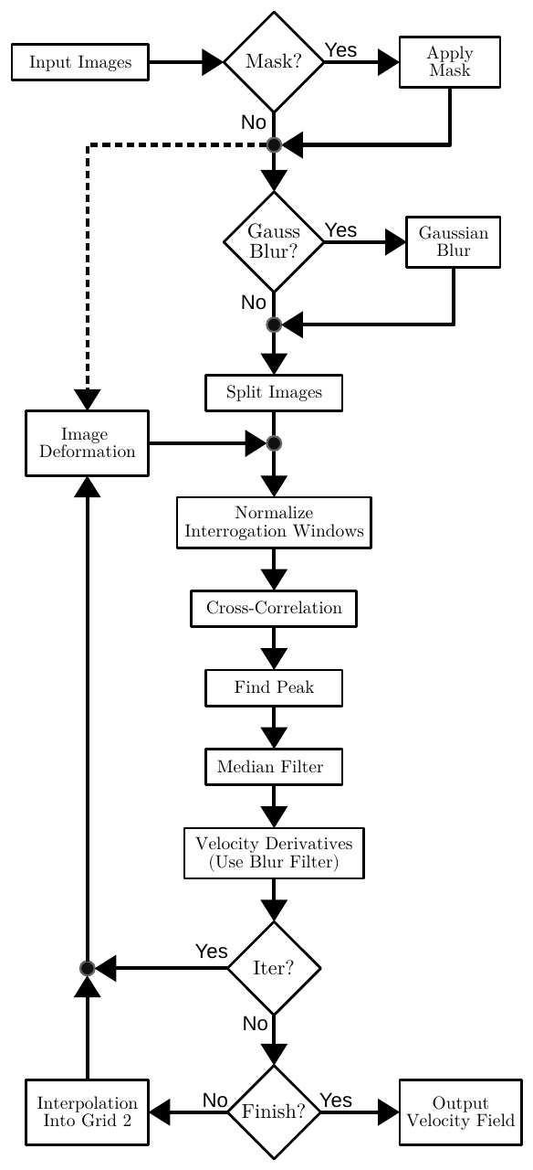
The DPIVSoft algorithm scheme (from the code paper, ref. 1).

Reading the boxes top to bottom, with the section and function implementing each one:

flowchart box	what it does	where
Apply Mask	zero solid regions; window-level mean fill	§7, masking/change_mask
Gaussian Blur	optional smoothing, first iteration only	§3.2, gaussian_filter
Split Images	cut both frames into the window grid	subimages
Normalize Interrogation Windows	subtract mean, scale by norm	§3, corrFFT*
Cross-Correlation	FFT (or direct) correlation per window pair	§3, corrFFT*/corrDirect1
Find Peak	peak selection + Westerweel correction + Gaussian sub-pixel fit	§4, find_peaks
Median Filter	reject vectors deviating from the neighbourhood median	§6, median_filter
Velocity Derivatives (Use Blur Filter)	smoothed gradients of the filtered field	§5.1, jacobian_matrix
Image Deformation	deform both frames by ∓u/2 → input for the next pass	§5.2, deform_image
Interpolation Into Grid 2	bi-linear interpolation of the converged field onto the finer grid	§5, interpolations

Two loops are nested: the inner Iter? loop repeats deform → correlate → update on the same grid until the residual converges; the outer Finish? loop switches from the coarse grid 1 to the fine grid 2 (the two-pass structure of §5).

---

3. Normalized cross-correlation of one window

For each interrogation window, take the two sub-images \(I_1, I_2\) (size \(B_x \times B_y\) pixels), subtract each one’s mean, and compute the normalized cross-correlation

\[ C(m, n) \;=\; \frac{\sum_{i,j} I_1'(i, j)\; I_2'(i + m,\, j + n)}{\sigma_1\, \sigma_2}, \qquad \sigma_k = \max\!\Big(0.1,\; \|I_k'\|\Big) \]

where \(I' = I - \bar{I}\) and \(\|I'\| = \sqrt{\sum I'^2}\). The maximum of \(C\) marks the most likely displacement of the particle pattern; the normalization makes peak heights comparable across windows regardless of local brightness, so a single noise-to-peak criterion can reject spurious vectors everywhere.

The correlation is evaluated by FFT (the whole sum for all shifts at once):

\[ C \;=\; \frac{\mathcal{F}^{-1}\!\left[\, \overline{\mathcal{F}(I_1')}\;\cdot\; \mathcal{F}(I_2') \,\right]}{\sigma_1\, \sigma_2} \]

followed by an FFT-shift so zero displacement sits at the window centre. The integer displacement is then

\[ u = m^\ast - B_x/2, \qquad v = n^\ast - B_y/2 \]

with \((m^\ast, n^\ast)\) the peak position. The search is restricted to a search window of size window_x × window_y around the centre (clipped to the box), which bounds the maximum detectable displacement and rejects far-off spurious peaks.

3.1 Direct correlation (direct_calc=True)

As an alternative for the first pass, corrDirect1() evaluates the correlation sum in physical space, only at the shifts inside the search window, re-normalizing both sub-images at every shift. It costs more per shift but computes far fewer shifts, and the per-shift re-normalization makes it more robust when large displacements push part of the pattern out of the window. The GPU pipeline implements the same option (directCorrelation / find_peak_direct kernels).

3.2 Optional image conditioning

• Gaussian pre-filter (gaussian_size > 0): both images are smoothed with a normalized Gaussian kernel before the first pass only — it raises the correlation peak of noisy or under-resolved particle images; the deformed passes go back to the raw images.

• Window weighting (weighting=True): a separable quadratic weight de-emphasizes pixels near the window edges, reducing the influence of particles entering/leaving the window.

---

4. Finding the peak with sub-pixel accuracy (find_peaks)

The raw peak position is integer-valued; PIV accuracy depends on locating it to a small fraction of a pixel.

Peak selection. The two highest local maxima inside the search window are found. Rather than keeping the taller one, the peak whose 3×3 neighbourhood carries the larger correlation sum is kept — a genuine displacement peak is broad (particle images have finite diameter), while noise spikes are narrow. If the second peak is too close in height to the first (ratio above peak_ratio), the window is ambiguous and the measurement is rejected (zeroed; the median filter of §6 then replaces it from the neighbours).

Westerweel bias correction. The correlation of finite windows is biased: at shift \((m, n)\) only a fraction of the two windows overlaps, attenuating the estimator by a triangular factor. Before the sub-pixel fit, each sample of the 3×3 neighbourhood is divided by

\[ \left(1 - \frac{|m|}{B_x}\right)\left(1 - \frac{|n|}{B_y}\right) \]

which removes the systematic pull of the peak toward zero displacement.

Three-point Gaussian fit (gauss_subpixel()). A well-resolved correlation peak is close to Gaussian, and a Gaussian through three points has a closed-form maximum. With \(a, b, c\) the correlation values at the peak’s left neighbour, the peak, and the right neighbour:

\[ \varepsilon \;=\; \frac{\ln a - \ln c}{2\left(\ln a + \ln c - 2 \ln b\right)} \qquad (-\tfrac12 < \varepsilon < \tfrac12) \]

applied independently in \(x\) and \(y\). The final window displacement is integer peak position + \(\varepsilon\) − window centre. The estimator is skipped (offset 0) when a sample is non-positive or the curvature is degenerate.

---

5. Multi-pass processing with window deformation

A single pass has two structural limitations: large boxes are needed to capture large displacements, but large boxes average over velocity gradients and lose spatial resolution. The classical cure is multi-pass processing with window deformation (Meunier & Leweke 2003), which is what processing() runs:

1. Pass 1 (coarse): correlate on a coarse grid (no_boxes_1_x × no_boxes_1_y boxes of box_size_1) without deformation → a robust but smoothed predictor field. Optionally iterate on this grid (no_iter_1 > 1) with median filtering + deformation (corrFFT1bis).

2. Pass 2 (fine): interpolate the predictor onto a finer grid (no_boxes_2_x × no_boxes_2_y, box_size_2, placed fully inside the first grid), then iterate deformation-correlation until sub-pixel convergence (corrFFT2).

5.1 The local velocity model

On the current grid, velocity gradients are computed by centred differences (one-sided at the borders) and smoothed with a 3×3 box filter (jacobian_matrix()). Inside window \((j, i)\), each pixel is assigned the linearised displacement

\[ u(i', j') = u_{ji} + \frac{\partial u}{\partial x}\,(i' - c_x) + \frac{\partial u}{\partial y}\,(j' - c_y) \]

(likewise for \(v\)), where \((c_x, c_y)\) is the window centre. This first-order expansion is what lets the method follow shear and rotation inside the window.

5.2 Symmetric deformation

Both sub-images are deformed by half the local displacement each, in opposite directions (deform_image() / translated_pixels(), bilinear interpolation):

\[ I_1 \text{ sampled at } \mathbf{x} - \tfrac{1}{2}\mathbf{u}(\mathbf{x}), \qquad I_2 \text{ sampled at } \mathbf{x} + \tfrac{1}{2}\mathbf{u}(\mathbf{x}) \]

This central-difference arrangement is second-order accurate: the correction is evaluated at the midpoint of the particle trajectory, not at one end. If the current field is exact, the deformed images coincide and the correlation peak sits exactly at zero — each pass measures only the residual error, and the update is

\[ u \leftarrow u_{\text{predicted at the peak pixel}} + \varepsilon + (m^\ast - B_x/2) \]

Displacements that would shift pixels outside the image are dropped (no shift in that direction) rather than extrapolated.

5.3 Convergence

The second pass repeats deform → correlate → update per window until the sub-pixel residual is below half a pixel or no_iter_2 iterations are reached. Because each iteration measures a residual, convergence is fast (2–3 iterations typical).

---

6. Validation: the median filter

Between iterations and at the end, median_filter() applies the classical median test: each vector is compared with the median of its 8 neighbours (reduced neighbourhoods at edges/corners), and vectors deviating by more than median_limit are replaced by the local median. This removes isolated outliers that survive peak selection — and, because deformation feeds the field back into the next iteration, it prevents one bad vector from corrupting its neighbourhood’s deformation.

---

7. Masks (solid regions)

A binary mask (Parameters.mask + mask image) excludes solid regions:

• The images are multiplied by the mask (masking()), zeroing solid pixels.

• Inside each window, masked pixels are replaced by the mean of the unmasked ones (change_mask()), so the mask edge itself does not correlate.

• Vectors whose window centre lies in the mask are zeroed (check_mask()), enforcing no-slip and stopping the median filter from bleeding values across the boundary.

---

8. Parameters

All options live in the global Parameters class (Classes.py), settable directly or loaded from YAML with Parameters.readParameters:

parameter	meaning
box_size_1_x/y, box_size_2_x/y	interrogation-window size, pass 1 / pass 2 (pixels)
no_boxes_1_x/y, no_boxes_2_x/y	grid size (number of windows), pass 1 / pass 2
window_1_x/y, window_2_x/y	correlation search-window size (pixels)
no_iter_1, no_iter_2	deformation iterations on grid 1 / grid 2
direct_calc	True = direct correlation on pass 1, False = FFT
median_limit	median-test rejection threshold
peak_ratio	max second/first peak-height ratio before rejection
gaussian_size	Gaussian pre-filter width (0 disables)
weighting	edge-de-emphasis window weighting (CPU only)
mask	enable solid-region masking

---

9. Practical use (CPU path)

import dpivsoft.DPIV as DPIV
from dpivsoft.Classes import Parameters

Parameters.readParameters("parameters.yaml")     # or set attributes directly

Img1, Img2 = DPIV.load_images("frame_a.png", "frame_b.png")
x, y, u, v = DPIV.processing(Img1, Img2)

DPIV.save(x, y, u, v, "result", 'openpiv')       # openpiv-compatible ASCII

Examples/simple_tutorial.py runs this end-to-end (synthetic image generation → CPU processing → GPU processing → saving); Examples/performance.py benchmarks CPU vs GPU.

---

10. Function reference

function	role
processing()	full two-pass pipeline on one image pair
corrFFT1()	pass 1: FFT correlation, no deformation
corrDirect1()	pass 1 alternative: direct correlation
corrFFT1bis()	extra deformation iterations on grid 1
corrFFT2()	pass 2: deformation iterations on the fine grid
find_peaks() / gauss_subpixel()	peak selection, Westerweel correction, sub-pixel fit
median_filter()	median-test outlier replacement
jacobian_matrix()	velocity gradients on the grid (centred + smoothed)
interpolations()	pass-1 field + gradients → pass-2 grid
deform_image() / translated_pixels()	symmetric window deformation (bilinear)
weight_function()	quadratic window weighting
gaussian_filter() / gaussian_kernel()	first-pass image smoothing
masking() / change_mask() / check_mask()	solid-region handling
load_images() / save()	I/O (grayscale float32; dpivsoft / openpiv / MATLAB formats)

---

References

1. J. Aguilar-Cabello, L. Parras, C. del Pino (2022), “DPIVSoft-OpenCL: A multicore CPU–GPU accelerated open-source code for 2D Particle Image Velocimetry,” SoftwareX 20, 101256, doi:10.1016/j.softx.2022.101256. — The code paper: this implementation, its OpenCL parallelisation and its validation; source of the algorithm scheme in §2.

2. P. Meunier, T. Leweke (2003), “Analysis and treatment of errors due to high velocity gradients in particle image velocimetry,” Exp. Fluids 35, 408–421. — The original DPIVSoft algorithm: multi-pass correlation with symmetric window deformation.

3. M. Raffel, C. E. Willert, S. T. Wereley, J. Kompenhans, Particle Image Velocimetry: A Practical Guide, 2nd ed., Springer (2007). — General reference for correlation PIV, peak fitting and post-processing.

4. J. Westerweel (1997), “Fundamentals of digital particle image velocimetry,” Meas. Sci. Technol. 8, 1379–1392. — Correlation-estimator bias and its correction.